Most explanations of cystic fibrosis flatten the problem too early.
"Less chloride" is true. It is also not enough.
"Bad channel" is true too. Still not enough.
I also built this because I have cystic fibrosis myself, and I wanted a lower-level way to understand what the disease was doing without stopping at the usual simplified summary.
What I wanted from this project was a way to force myself to understand CFTR at a lower mechanistic level in a format that works for how my brain thinks. That meant writing code. Not reading another summary. Not memorising another pathway diagram. I wanted a hidden-state model I could build, fit, inspect, and break.
So I built a continuous-time hidden Markov inference pipeline for CFTR gating. It takes a trace, fits a generator matrix , decodes latent-state occupancy, computes implied relaxation times from the spectrum, and turns the whole thing back into a story about how probability flows through a compact gating topology.
The point was never to produce a clinical tool or pretend I had a publication-grade medical inference engine. The point was to make CFTR legible as a stochastic dynamical system. For that, this project did exactly what I needed it to do.
Just as importantly, the outputs I discuss here are from a deliberately small illustrative subset that was fast enough to iterate on, inspect, and mentally parse. They are not meant to stand in for a full long-run fit on every available trace.
Why I modeled CFTR this way
Patch clamp gives you a scalar current trace:
CFTR does not live in scalar-current space. It lives in hidden conformational states and moves between them stochastically. The amplifier sees the consequences of those hidden transitions, not the states themselves.
That immediately forces a two-layer model:
- a hidden kinetic system
- an observation model
I used a continuous-time Markov chain for the hidden kinetics. With the column-vector convention I used in code, the state probability vector evolves as
with generator matrix satisfying
and column conservation
Sampling happens on a discrete grid, so the continuous-time kinetics have to be bridged into a discrete transition matrix:
That is the whole hinge of the project. The kinetics stay continuous-time. The inference stays in a discrete HMM-style form that I can actually compute.
This framing matters because it changes how CF looks. Instead of "does the channel open enough," the question becomes "how does probability flow through the hidden gating architecture?" That is a much better question.
The 4-state model
I started with the smallest topology that still gave me the pieces I cared about:
In code, that topology is hard-coded in src/main.cpp:
1Eigen::MatrixXi make_cftr4_topology()
2{
3    Eigen::MatrixXi topology = Eigen::MatrixXi::Zero(4, 4);
4    topology(1, 0) = 1; // CI -> CB
5    topology(0, 1) = 1; // CB -> CI
6    topology(2, 1) = 1; // CB -> O
7    topology(1, 2) = 1; // O -> CB
8    topology(3, 2) = 1; // O -> F
9    topology(2, 3) = 1; // F -> O
10    return topology;
11}
That gives the 4-state generator
This is the first place where the project started teaching me something useful.
In the code, those names are topology labels attached to states 0,1,2,3. They are not enforced identifiability constraints. The topology distinguishes a long-range closed state, an intermediate closed state, and two more open-adjacent states, but after fitting I still have to be careful: without an explicit relabelling rule, the latent states are fundamentally indexed states first and biological interpretations second.
Parameterising so it stays valid
Before I touched likelihood or decoding, I wanted the generator itself to be impossible to break by construction.
So I kept the off-diagonal rates in unconstrained log-space and rebuilt the diagonals from the column sums. In src/GeneratorMatrix.cpp:
1for (int from = 0; from < n_; ++from)
2{
3    for (int to = 0; to < n_; ++to)
4    {
5        if (from == to || !allowed_(to, from))
6        {
7            continue;
8        }
9
10        Q_(to, from) = std::exp(beta_(idx));
11        ++idx;
12    }
13}
14
15for (int col = 0; col < n_; ++col)
16{
17    const double off_diag_sum = Q_.col(col).sum() - Q_(col, col);
18    Q_(col, col) = -off_diag_sum;
19}
Mathematically that is
with
That bought me three useful things immediately:
- allowed rates stay positive
- forbidden edges stay exactly zero
- the optimiser gets an unconstrained parameter space
For the 4-state model there are six directed rates, so the kinetic block of the parameter vector is six-dimensional.
From kinetics to samples
Once I had , I needed the discrete transition operator at the sampling interval. I did not try to get fancy here. src/GeneratorMatrix.cpp just uses Eigen's matrix exponential:
1Eigen::MatrixXd GeneratorMatrix::transition_matrix(double dt) const
2{
3    if (dt < 0.0)
4    {
5        throw std::runtime_error("dt must be nonnegative");
6    }
7    return (Q_ * dt).exp();
8}
For a hidden kinetic model, that was the right tradeoff. It is simple, readable, and good enough to keep the focus where I wanted it: on the gating logic, not on reimplementing matrix-function numerics.
The observation model
I used Gaussian emissions:
So
That lives in src/EmissionModel.cpp:
1const double sigma = std::max(sigma_(state), config::kRateFloor);
2const double diff = y - mu_(state);
3const double variance = sigma * sigma;
4return -0.5 * std::log(kTwoPi * variance) - (diff * diff) / (2.0 * variance);
This is another place where the hidden-state framing matters. Two states can be electrically similar but kinetically different. That is exactly why an HMM is useful here. You do not build a hidden-state model because the states are obvious. You build it because they are not.
The likelihood
The complete-data likelihood for a hidden path is
With the current implementation, the initial distribution is fixed rather than optimised. So the observed-data likelihood is
That is impossible to compute by explicit enumeration once the trace gets long, so the project uses forward-backward.
I packed the optimisation vector as
That unpacking happens in src/Likelihood.cpp:
1const Eigen::VectorXd beta = x.head(rate_params);
2const Eigen::VectorXd mu = x.segment(rate_params, n);
3const Eigen::VectorXd log_sigma = x.tail(n);
4const Eigen::VectorXd sigma = log_sigma.array().exp().max(config::kRateFloor).matrix();
For the 4-state model:
free parameters.
That exact parameter count shows up later in the AIC/BIC model-comparison outputs.
Forward-backward and Viterbi
The scaled forward recursion is
At each step I scale:
Then
In code, src/ForwardBackward.cpp does exactly that:
1for (int k = 1; k < T; ++k)
2{
3    for (int i = 0; i < n; ++i)
4    {
5        const double predicted = A.row(i).dot(result.alpha.col(k - 1));
6        result.alpha(i, k) = emission.pdf(i, trace.samples[k].y) * predicted;
7    }
8
9    scale[k] = std::max(result.alpha.col(k).sum(), config::kProbEpsilon);
10    result.alpha.col(k) /= scale[k];
11    result.log_likelihood += std::log(scale[k]);
12}
Backward messages and posteriors follow:
Then I added Viterbi to get a single most likely hidden path:
This is implemented in src/Viterbi.cpp:
1const double aji = std::max(A(i, j), config::kProbEpsilon);
2const double candidate = delta(j, k - 1) + std::log(aji);
3if (candidate > best)
4{
5    best = candidate;
6    arg_best = j;
7}
8delta(i, k) = best + emission.log_pdf(i, trace.samples[k].y);
The important thing this gave me was not just a best path. It gave me a way to see the hidden gating regimes directly in the trace.
The optimiser
The optimiser in this project is not glamorous. src/OptimizerFacade.cpp is finite-difference gradient descent with backtracking line search.
1const double h = 1e-4 * (1.0 + std::abs(x(i)));
2...
3grad(i) = (fp - fm) / (2.0 * h);
then
1const Eigen::VectorXd direction = -grad;
2double step = 1.0;
3while (step >= min_step)
4{
5    const Eigen::VectorXd candidate = x + step * direction;
6    const double f_candidate = f(candidate);
7    if (std::isfinite(f_candidate) && f_candidate < fx)
8    {
9        x = candidate;
10        fx = f_candidate;
11        improved = true;
12        break;
13    }
14    step *= 0.5;
15}
This is not a production optimiser. It was enough to get the system moving and, more importantly, enough to let me see the hidden-state structure emerge. That was the point.
Spectral decomposition
Once I had a fitted generator, the spectrum was the part that made the system feel dynamically readable.
Numerically, the code computes the eigenvalues of and reports relaxation times from their real parts. Formally, if is diagonalizable and
then for each eigenvalue with negative real part it reports
That is the quantity computed in src/SpectralAnalysis.cpp:
1const double re = eig(i).real();
2const double im = eig(i).imag();
3double tau = std::numeric_limits<double>::infinity();
4if (std::abs(re) > eps && re < 0.0)
5{
6    tau = -1.0 / re;
7}
With the same column-vector convention, the stationary distribution is recovered from the normalised null-space condition
Operationally, the code solves a normalised linear system built from that condition, clips small negative numerical artefacts to zero, and renormalises.
In the wild-type phase 7 spectrum output, the fitted finite relaxation times are:
- slow mode:
1.61751 s - intermediate mode:
0.495865 s - fast mode:
0.281996 s
That was exactly the kind of thing I wanted out of the project. The hidden gating dynamics stop looking like a binary switch and start looking like layered relaxation processes.
At the same time, these should be read carefully. The example traces discussed here are short, deliberately chosen illustrative inputs, so these are model-implied relaxation times from the fitted , not directly resolved kinetic measurements.
Model comparison
I did not want to just decide that 4-state was the answer and never test it.
So the project compares a small candidate set using
Because the code optimises negative log-likelihood,
the implemented forms are
That is exactly what compare_models_on_trace() writes out.
One important detail: this is not a pure "state count only" comparison. The 4-state candidate uses the hand-specified CFTR burst-flicker topology above, while the 2-, 3-, and 5-state candidates are simple bidirectional chains. So the comparison is over a small set of state-count-and-topology pairs, not over every possible -state architecture.
For the phase 7 condition bundle, the 4-state model wins by BIC in all three conditions:
| Condition | 2-state BIC | 3-state BIC | 4-state BIC | 5-state BIC | Winner |
|---|---|---|---|---|---|
| wild type | -32.4193 | 5.4290 | -159.5340 | -138.1480 | 4-state |
| mutant | -18.9370 | -1.3151 | -56.1140 | -20.6382 | 4-state |
| drug treated | -122.4020 | -99.8955 | -130.9960 | -75.5548 | 4-state |
That matters because it means this particular 4-state topology is not just me insisting on complexity for aesthetic reasons. Within the candidate set implemented in the project, it is the BIC winner on all three included phase 7 conditions.
What the wild-type decoding actually looks like
The most useful outputs in the whole project ended up being the decoded wild-type figures.
The posterior CSV results/phase7/decode/wild_type_posteriors.csv shows mean posterior occupancy over the indexed latent states, using the topology labels only as shorthand:
- state
0(CIlabel): about0.076 - state
1(CBlabel): about0.370 - state
2(Olabel): about0.553 - state
3(Flabel): essentially0
The Viterbi path in results/phase7/decode/wild_type_viterbi_path.csv is even cleaner:
- state
0(CI) dominates the first 12 samples - state
1(CB) then takes over - state
2(O) dominates the longest stretches - state
3(F) is effectively unused in this trace
The corresponding preprocessed trace starts negative and low, then rises steadily:
1time,current
20,-0.23856
30.0015,-0.234331
40.003,-0.237309
5...
60.018,0.219119
70.0195,0.320376
80.021,0.430991
90.0225,0.513907
100.024,0.593103
110.0255,0.639474
120.027,0.684196
What that gave me was a lower-level picture of the fitted latent dynamics that felt much more real than just "the current rose."
In this example, the decoded path starts in state 0, moves through state 1, and then spends most of its time in state 2. I can interpret that as a progression from lower-current to higher-current occupancy, but the code itself only guarantees the indexed latent-state sequence, not a uniquely identified biological labelling.
Condition summaries
The phase 7 summary table is:
$P_{2,3}means stationary occupancy of latent states{2,3}Occupancy_{1,2,3}means stationary occupancy of latent states{1,2,3}Mean run duration_{2,3}means the mean contiguous Viterbi run duration in states{2,3}Rate 2 -> 3andRate 3 -> 2are the corresponding fitted generator entries by state index
| Condition | Samples P2,3 | Occupancy 1,2,3 | Mean run duration 2,3 (s) | Run count / s 2,3 | Slowest mode (s) | Third sorted mode by |Re(λ)| (s) | Rate 2→3 | Rate 3→2 |
|---|---|---|---|---|---|---|---|---|
| wild type | 151 | 0.505361 | 0.758173 | 0.06300 | 8.83002 | 1.61751 | 0.495865 | 0.994616 |
| mutant | 65 | 0.528072 | 0.781567 | 0.04650 | 10.2564 | 1.49329 | 0.473645 | 1.032620 |
| drug treated | 227 | 0.484723 | 0.738802 | 0.04575 | 5.87372 | 1.62218 | 0.475260 | 0.995543 |
These are not numbers I would present as definitive biological estimates. That is not what this project was for. They come from a compact, intentionally small subset that was useful for understanding the machinery without waiting on full-scale runs, and they should be read as model-conditioned summaries for that subset. What they are useful for is something more foundational: they show the kind of quantities the fitted hidden-state system exposes once you stop thinking about CFTR as a binary channel and start thinking about it as a stochastic kinetic model.
State occupancies are there. Run durations are there. Exchange rates between indexed latent states are there. The slow mode is there. That is the conceptual win.
The plots were part of the point
The CSV outputs were useful, but the plots were what really made the model click for me.
Seeing the posterior mass move between latent states over time made the hidden-state idea feel concrete instead of abstract. The model stopped being "some likelihood function I fit" and started looking like an actual evolving explanation of the trace.
Posterior occupancy over time
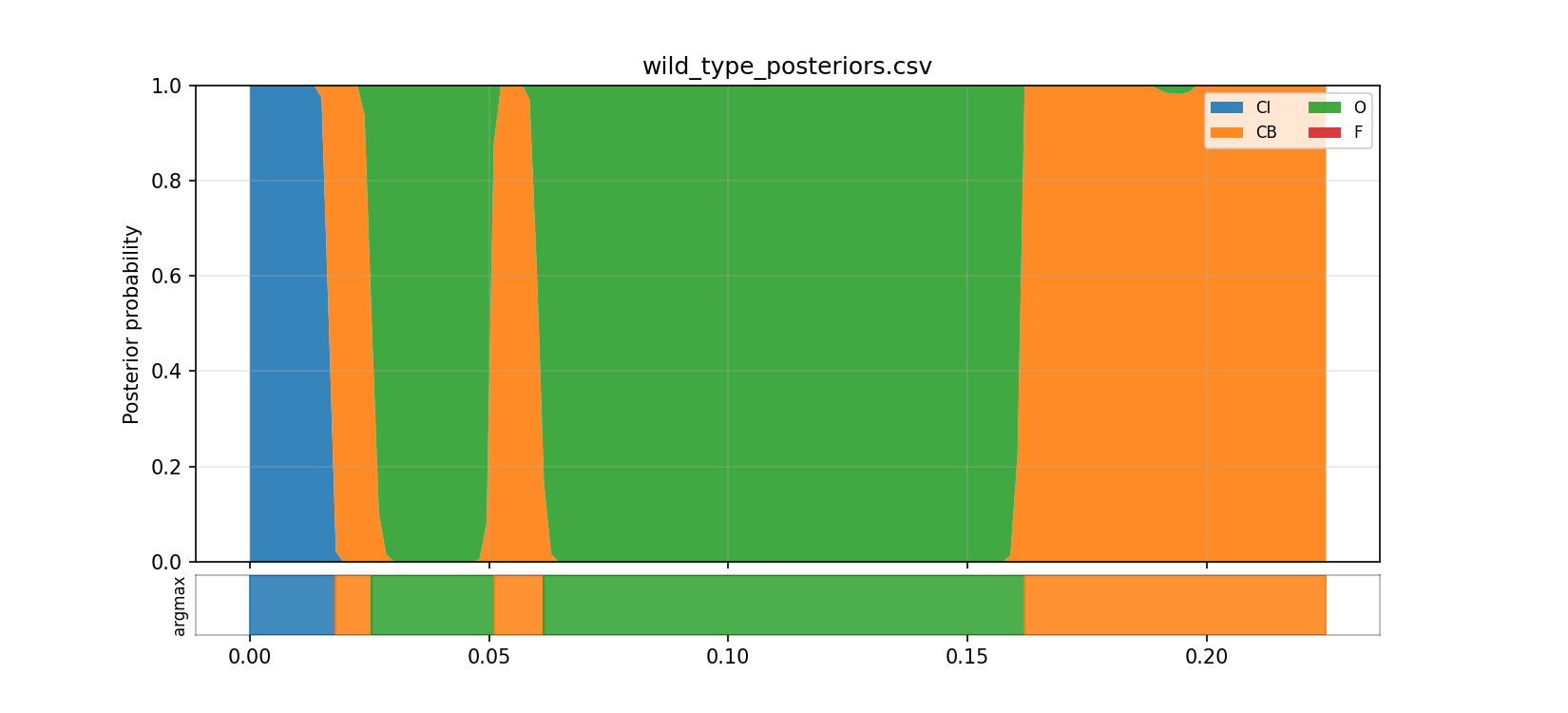
This is the picture that made the HMM interpretation feel real to me. Instead of one current value at each time point, I can see the model's uncertainty distributed across latent states and watch that distribution shift through the trace.
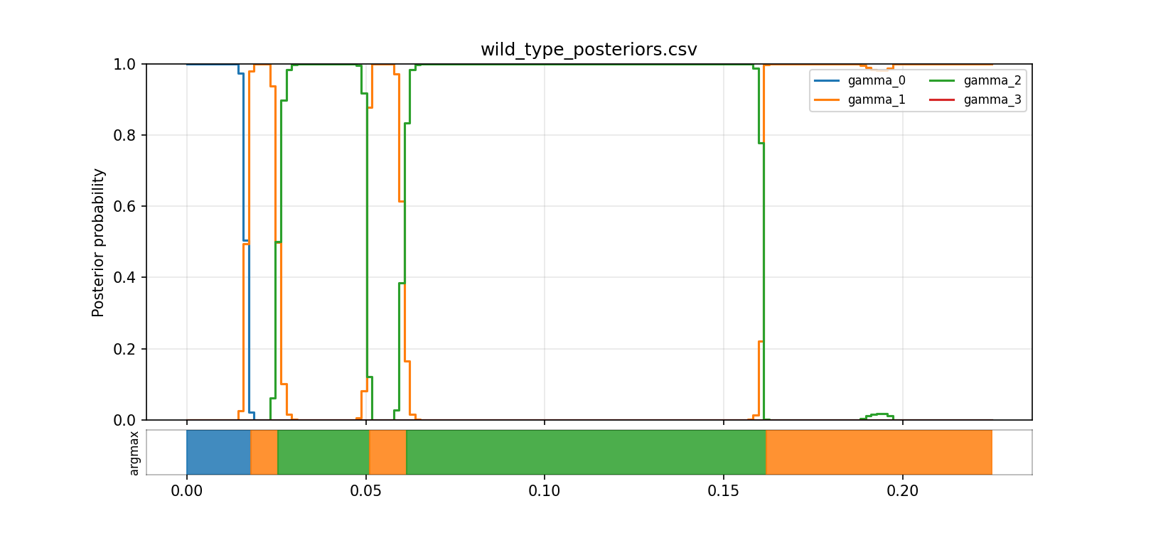
The step view makes it easier to see where one latent state starts to dominate and where the model stays uncertain. Even without claiming that every state has a uniquely identified biological meaning, this is already much more informative than treating the trace as a simple open/closed line.
Decoded trace overlay
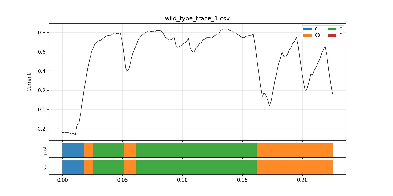
This overlay was useful because it let me compare the raw current trajectory against the inferred latent-state structure in the same frame. It is the point where the model stopped feeling like detached math and started feeling like an interpretable readout of the trace.
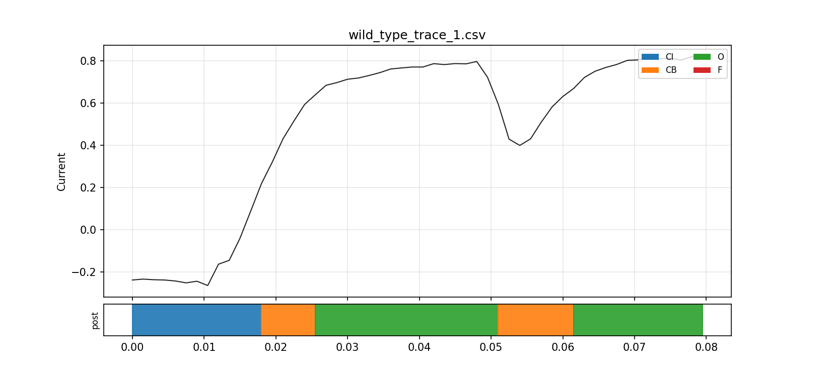
The zoomed view is even better for intuition. It shows the local transitions and makes it much easier to see how the fitted state sequence relates to rises, plateaus, and brief shifts in the observed current.
Spectrum plots
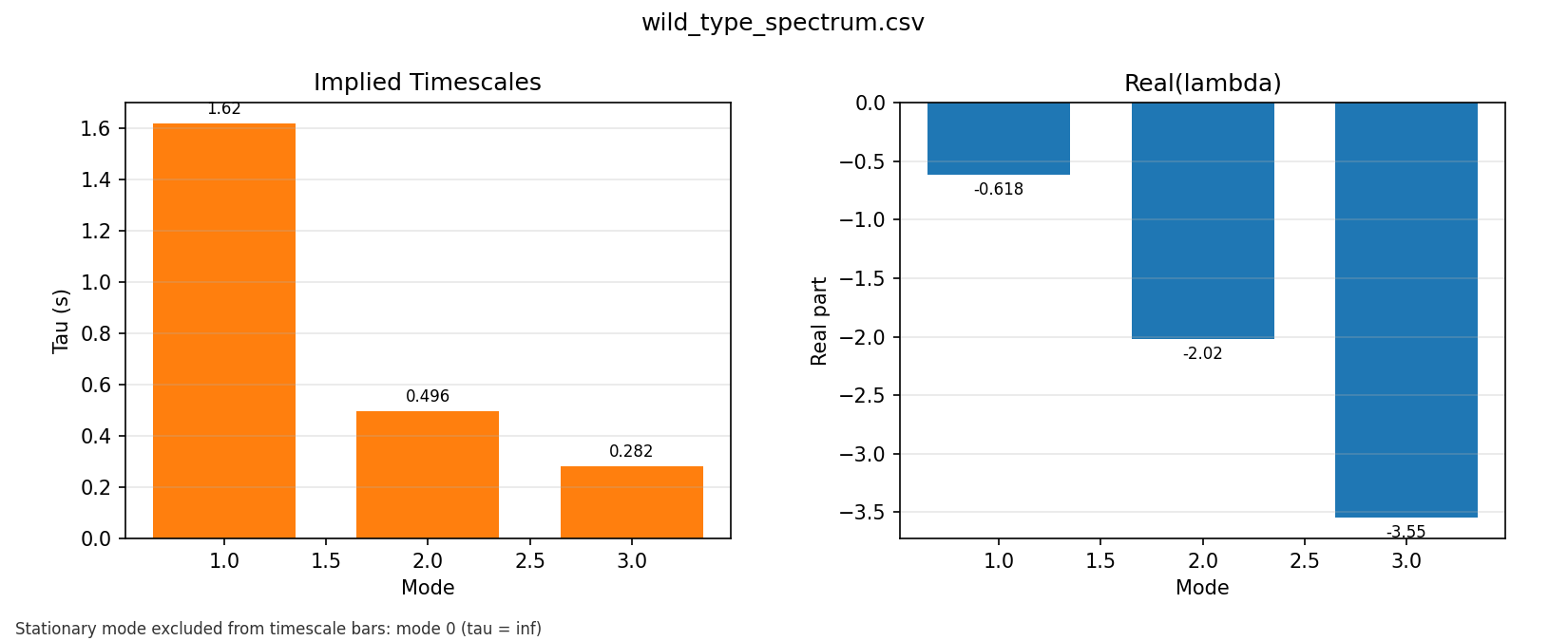
The spectrum plot turns the fitted generator into a timescale picture. That helped me see the model less as a list of rates and more as a layered dynamical system with slow and fast relaxation structure.
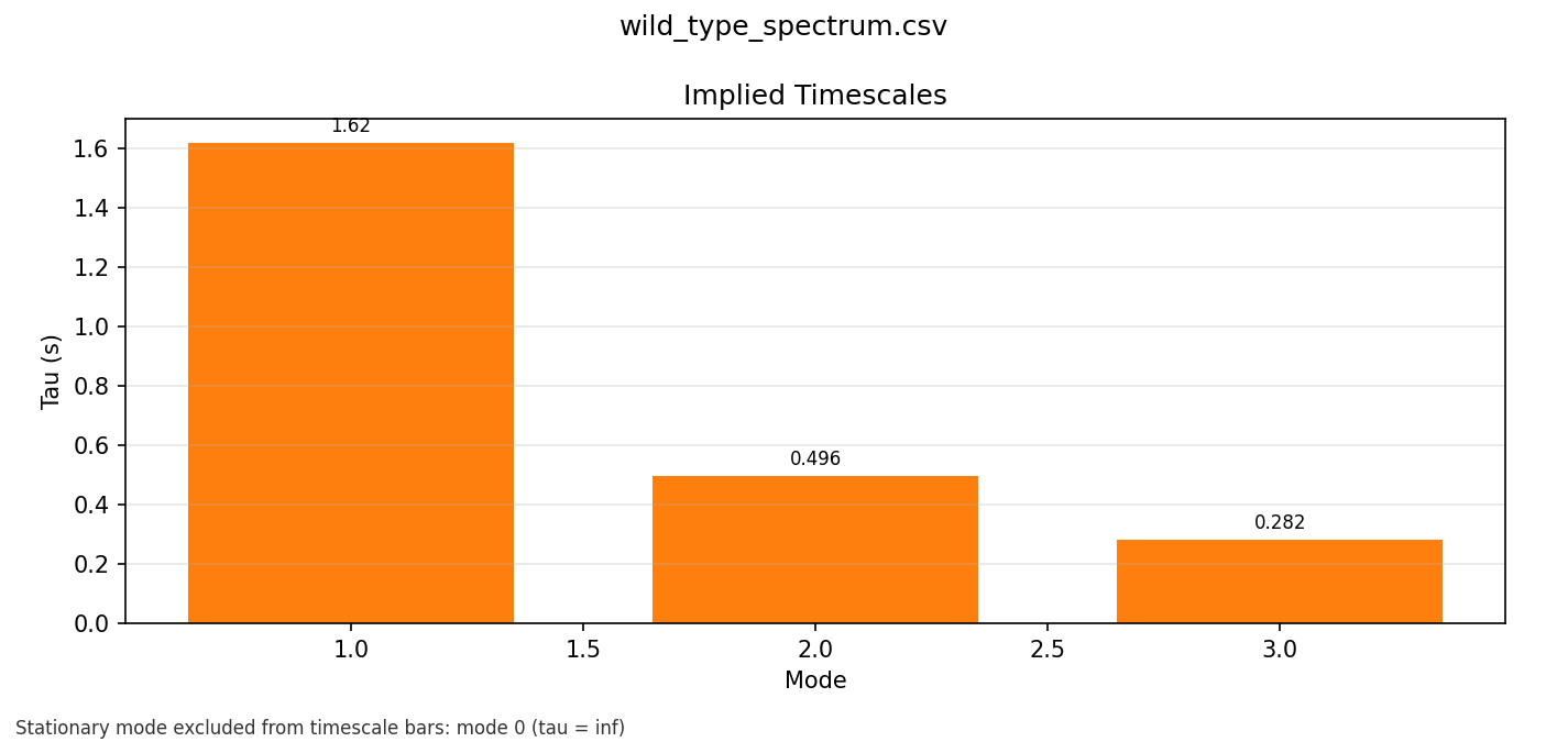
This was another conceptual unlock for me: once the fitted process is summarised in terms of characteristic timescales, it becomes much easier to reason about what parts of the dynamics are slow, what parts are fast, and why a binary mental model leaves too much out.
What this project taught me about cystic fibrosis
The most useful thing this project did was change what I think the object of explanation is.
Before building this, it is easy to let CF collapse into a story like:
- less chloride
- less opening
- bad protein
After building this, that feels too flat.
The more useful picture is:
- CFTR occupies hidden gating states
- function depends on how probability moves between them
- mutations and rescue can shift occupancy, transition bias, and timescale structure
- open probability is one consequence of that hidden dynamics, not the whole thing
That is the lower-level lesson I wanted.
CF starts to look less like a scalar defect and more like a distortion of stochastic flow through a compact state machine.
That is a much better mental model.
A brief honesty note
I am not presenting this as medical research. I am not pretending the fitted values here are definitive biological measurements. The point of the project was to build a working hidden-state model that makes CFTR legible as a stochastic dynamical system. For that, the model succeeds.
The exact fitted values are not the point. The point is that even a compact, computationally tractable model is enough to surface hidden structure in occupancy, transition balance, and relaxation times instead of collapsing everything into a flatter "bad channel" story.
The phase 7 results shown here should be read for what they are: a small illustrative subset used to understand the model behaviour without paying the runtime cost of full long-recording fits. They are useful for intuition, code inspection, and stress-testing the pipeline, not for claiming that a particular fitted latent state has a uniquely established biological identity or that the reported numbers are final full-dataset estimates.
The model itself also bakes in choices that matter: a fixed candidate topology set, a fixed initial-state prior during fitting, Gaussian emissions, and index-based summary metrics unless an explicit relabelling step is added. So the outputs are best read as "what this implementation reports under these assumptions" rather than as assumption-free facts about CFTR.
That is what I needed this project to show me, and that is what it showed.